Economic Impact Assessment: How much is a project really worth to the economy?

A research centre in Ireland took in €98.69 million over thirteen years. Its contribution to the Irish economy over the same period: €515.32 million. Numbers like these decide funding, planning and policy. This guide explains how they are calculated, and how to tell a credible one from an inflated one. MCC Economics carries out these assessments for governments and companies in the United Kingdom, Ireland and the Gulf. The full 21-page article below draws on 26 sources across three economies, and every figure on this page traces to the sources listed in the references.

Quick Answer

An Economic Impact Assessment measures the effect of a project, company or investment on the economy of a defined area, counting the direct activity, the supply chain it supports, and the spending of the wages it pays. It matters because a project’s full contribution is larger than its own accounts show, and funding decisions depend on the full number.

Key Takeaways

  • An Economic Impact Assessment measures a project’s effect on a defined area’s economy in three categories: direct effects from the activity itself, indirect effects along its supply chain, and induced effects from employees spending their wages locally.
  • Economic multipliers express how far each unit of direct activity ripples outward, and they come in two types: Type I covers direct and indirect effects only, while Type II adds induced effects, which is why this guide recommends Type II for a complete picture.
  • Practical multipliers are built from input-output models, tables published by national statistics offices, such as the Scottish Government and Ireland’s Central Statistics Office, that map how money flows between every sector of an economy.
  • A credible assessment nets off deadweight, the activity that would have happened anyway, so the final number reflects what the project genuinely added rather than everything that occurred around it.
  • The method scales to whole industries: Oxford Economics found the UAE aluminium sector contributed US $5.47 billion to the national economy in 2017, with every US $1 of the sector’s own GDP supporting a further US $1.26 elsewhere.

What is an Economic Impact Assessment?

An Economic Impact Assessment (EIA) measures the effect of an economic event or activity on the economy of a specified area. The subject can be a company, an investment project or a whole sector. This is the economic EIA, not the environmental impact assessment that shares the acronym: the economic kind deals in output, incomes and jobs rather than habitats and emissions.

The impacts are usually measured in monetary values, such as total output, GDP, Gross Value Added (a project’s direct contribution to GDP) and total household earnings, or in real-world outcomes, most commonly the change in the number of jobs. Whichever measures are chosen, the purpose is the same: to capture in full what an activity contributes to the economy around it, not only what appears in its own accounts.

That wider contribution falls into three categories, and the guide treats all three as equally important: direct, indirect and induced effects, which the next section takes in turn. The method is practical rather than theoretical: this guide works through three applications at three different scales, a single research centre in Ireland assessed over thirteen years, an entire industrial sector in the United Arab Emirates assessed by Oxford Economics, and the official input-output tables published by the Scottish Government, which are the foundation such assessments are built on.

What are direct, indirect and induced economic effects?

Direct effects are the contribution that comes straight from the subject’s own activity: its output, the people it employs, the value it adds. Indirect effects are the contributions that result from the subject’s impact on the firms and sectors related to it, measured all along its supply chain. Induced effects arise from the subject’s activity without being related to it: the classic example is the increase in revenue of local grocery stores once the people employed by the subject begin receiving and spending their salaries.

The three layers matter because each answers a different question. Direct effects show what the project is; indirect effects show what it buys; induced effects show what its wages do in the local economy. A complete assessment counts all three.

What is an economic multiplier?

An economic multiplier is a ratio that shows the total effect on the economy of one extra unit of activity, for example one extra pound of spending or investment. Two textbook examples illustrate the idea. The Keynesian multiplier, 1 / (1 − MPC), where MPC is the marginal propensity to consume, the share of each extra unit of income that people spend rather than save, measures the impact on GDP of changes in private investment or government spending. The bank multiplier, also called the deposit or money multiplier, is 1 / RR, where RR is the reserve requirement, the share of every deposit that banks must keep at the central bank rather than lend out. It shows how much money the banking system can create from each deposit.

Both are theoretical: the simplifying assumptions behind them mean they can hardly be applied in a real analysis. Their principles carry over, though, and practical assessments build industry-specific and economy-specific multipliers instead, usually from an input-output model.

What is the difference between Type I and Type II multipliers?

Type I multipliers cover direct and indirect effects only; Type II multipliers add induced effects as well. A Type I multiplier estimates the ripple down the supply chain: a producer increases output to meet new demand, buys more from its suppliers, who buy more from theirs, and so on. Because it stops there, a Type I multiplier underestimates the effect on the economy. A Type II multiplier also counts the local spending of employees’ wages, and is calculated as the ratio of direct, indirect and induced effects together to direct effects alone. For a complete picture of a project’s impact, this guide recommends Type II.

“Type I multipliers underestimate the effect on the economy as they do not estimate induced effects.”

How do input-output models turn data into multipliers?

An input-output (IO) model is a detailed map of an economy, built from data, showing how every sector buys from and sells to every other, so that the output of one sector becomes an input to another. In the model’s central table, the inter-industry matrix, columns show what a sector buys and rows show what it sells, revealing how dependent each sector is on all the rest.

Figure 1: The hypothetical transactions table from the source article, reproduced in its original format with all its values, six industries, final demand and the payments rows.

Hypothetical Transactions Table

Industry Purchasing

Industry Producing  Processing SectorPayments Sector
Processing SectorFinal Demand
Outputs¹ →
Inputs² ↓
(1)
A
(2)
B
(3)
C
(4)
D
(5)
E
(6)
F
(7)
Gross inventory accumula-tion (+)
(8)
Exports to foreign countries
(9)
Government purchases
(10)
Gross private capital formation
(11)
Households
(12)
Total Gross Output
(1) Industry A10Industry A uses 10 of its own output.15Industry A sells 15 to Industry B; equally, B buys 15 from A.1Industry A sells 1 to Industry C; equally, C buys 1 from A.2Industry A sells 2 to Industry D; equally, D buys 2 from A.5Industry A sells 5 to Industry E; equally, E buys 5 from A.6Industry A sells 6 to Industry F; equally, F buys 6 from A.2Industry A sells 2 to final demand: gross inventory accumulation.5Industry A sells 5 to final demand: exports to foreign countries.1Industry A sells 1 to final demand: government purchases.3Industry A sells 3 to final demand: gross private capital formation.14Industry A sells 14 to final demand: households.64Everything Industry A sells across the row: total gross output of 64.
(2) Industry B5Industry B sells 5 to Industry A; equally, A buys 5 from B.4Industry B uses 4 of its own output.7Industry B sells 7 to Industry C; equally, C buys 7 from B.1Industry B sells 1 to Industry D; equally, D buys 1 from B.3Industry B sells 3 to Industry E; equally, E buys 3 from B.8Industry B sells 8 to Industry F; equally, F buys 8 from B.1Industry B sells 1 to final demand: gross inventory accumulation.6Industry B sells 6 to final demand: exports to foreign countries.3Industry B sells 3 to final demand: government purchases.4Industry B sells 4 to final demand: gross private capital formation.17Industry B sells 17 to final demand: households.59Everything Industry B sells across the row: total gross output of 59.
(3) Industry C7Industry C sells 7 to Industry A; equally, A buys 7 from C.2Industry C sells 2 to Industry B; equally, B buys 2 from C.8Industry C uses 8 of its own output.1Industry C sells 1 to Industry D; equally, D buys 1 from C.5Industry C sells 5 to Industry E; equally, E buys 5 from C.3Industry C sells 3 to Industry F; equally, F buys 3 from C.2Industry C sells 2 to final demand: gross inventory accumulation.3Industry C sells 3 to final demand: exports to foreign countries.1Industry C sells 1 to final demand: government purchases.3Industry C sells 3 to final demand: gross private capital formation.5Industry C sells 5 to final demand: households.40Everything Industry C sells across the row: total gross output of 40.
(4) Industry D11Industry D sells 11 to Industry A; equally, A buys 11 from D.1Industry D sells 1 to Industry B; equally, B buys 1 from D.2Industry D sells 2 to Industry C; equally, C buys 2 from D.8Industry D uses 8 of its own output.6Industry D sells 6 to Industry E; equally, E buys 6 from D.4Industry D sells 4 to Industry F; equally, F buys 4 from D.0Industry D sells 0 to final demand: gross inventory accumulation.0Industry D sells 0 to final demand: exports to foreign countries.1Industry D sells 1 to final demand: government purchases.2Industry D sells 2 to final demand: gross private capital formation.4Industry D sells 4 to final demand: households.39Everything Industry D sells across the row: total gross output of 39.
(5) Industry E4Industry E sells 4 to Industry A; equally, A buys 4 from E.0Industry E sells 0 to Industry B; equally, B buys 0 from E.1Industry E sells 1 to Industry C; equally, C buys 1 from E.14Industry E sells 14 to Industry D; equally, D buys 14 from E.3Industry E uses 3 of its own output.2Industry E sells 2 to Industry F; equally, F buys 2 from E.1Industry E sells 1 to final demand: gross inventory accumulation.2Industry E sells 2 to final demand: exports to foreign countries.1Industry E sells 1 to final demand: government purchases.3Industry E sells 3 to final demand: gross private capital formation.9Industry E sells 9 to final demand: households.40Everything Industry E sells across the row: total gross output of 40.
(6) Industry F2Industry F sells 2 to Industry A; equally, A buys 2 from F.6Industry F sells 6 to Industry B; equally, B buys 6 from F.7Industry F sells 7 to Industry C; equally, C buys 7 from F.6Industry F sells 6 to Industry D; equally, D buys 6 from F.2Industry F sells 2 to Industry E; equally, E buys 2 from F.6Industry F uses 6 of its own output.2Industry F sells 2 to final demand: gross inventory accumulation.4Industry F sells 4 to final demand: exports to foreign countries.2Industry F sells 2 to final demand: government purchases.1Industry F sells 1 to final demand: gross private capital formation.8Industry F sells 8 to final demand: households.46Everything Industry F sells across the row: total gross output of 46.
(7) Gross inventory depletion (−)1Inventory drawn down: 1 in Industry A’s column of inputs.2Inventory drawn down: 2 in Industry B’s column of inputs.1Inventory drawn down: 1 in Industry C’s column of inputs.0Inventory drawn down: 0 in Industry D’s column of inputs.2Inventory drawn down: 2 in Industry E’s column of inputs.1Inventory drawn down: 1 in Industry F’s column of inputs.0Inventory drawn down: 0 against gross inventory accumulation.1Inventory drawn down: 1 against exports to foreign countries.0Inventory drawn down: 0 against government purchases.0Inventory drawn down: 0 against gross private capital formation.0Inventory drawn down: 0 against households.8Inventory drawn down: 8 across the whole economy.
(8) Imports2Inputs bought from abroad, which leak out of the domestic economy: 2 in Industry A’s column of inputs.1Inputs bought from abroad, which leak out of the domestic economy: 1 in Industry B’s column of inputs.3Inputs bought from abroad, which leak out of the domestic economy: 3 in Industry C’s column of inputs.0Inputs bought from abroad, which leak out of the domestic economy: 0 in Industry D’s column of inputs.3Inputs bought from abroad, which leak out of the domestic economy: 3 in Industry E’s column of inputs.2Inputs bought from abroad, which leak out of the domestic economy: 2 in Industry F’s column of inputs.0Inputs bought from abroad, which leak out of the domestic economy: 0 against gross inventory accumulation.0Inputs bought from abroad, which leak out of the domestic economy: 0 against exports to foreign countries.0Inputs bought from abroad, which leak out of the domestic economy: 0 against government purchases.0Inputs bought from abroad, which leak out of the domestic economy: 0 against gross private capital formation.2Inputs bought from abroad, which leak out of the domestic economy: 2 against households.13Inputs bought from abroad, which leak out of the domestic economy: 13 across the whole economy.
(9) Payments to government2Taxes and payments to government: 2 in Industry A’s column of inputs.3Taxes and payments to government: 3 in Industry B’s column of inputs.2Taxes and payments to government: 2 in Industry C’s column of inputs.2Taxes and payments to government: 2 in Industry D’s column of inputs.1Taxes and payments to government: 1 in Industry E’s column of inputs.2Taxes and payments to government: 2 in Industry F’s column of inputs.3Taxes and payments to government: 3 against gross inventory accumulation.2Taxes and payments to government: 2 against exports to foreign countries.1Taxes and payments to government: 1 against government purchases.2Taxes and payments to government: 2 against gross private capital formation.12Taxes and payments to government: 12 against households.32Taxes and payments to government: 32 across the whole economy.
(10) Depreciation allowances1Depreciation set aside: 1 in Industry A’s column of inputs.2Depreciation set aside: 2 in Industry B’s column of inputs.1Depreciation set aside: 1 in Industry C’s column of inputs.0Depreciation set aside: 0 in Industry D’s column of inputs.1Depreciation set aside: 1 in Industry E’s column of inputs.0Depreciation set aside: 0 in Industry F’s column of inputs.0Depreciation set aside: 0 against gross inventory accumulation.0Depreciation set aside: 0 against exports to foreign countries.0Depreciation set aside: 0 against government purchases.0Depreciation set aside: 0 against gross private capital formation.0Depreciation set aside: 0 against households.5Depreciation set aside: 5 across the whole economy.
(11) Households19Wages and income paid to households: 19 in Industry A’s column of inputs.23Wages and income paid to households: 23 in Industry B’s column of inputs.7Wages and income paid to households: 7 in Industry C’s column of inputs.5Wages and income paid to households: 5 in Industry D’s column of inputs.9Wages and income paid to households: 9 in Industry E’s column of inputs.12Wages and income paid to households: 12 in Industry F’s column of inputs.1Wages and income paid to households: 1 against gross inventory accumulation.0Wages and income paid to households: 0 against exports to foreign countries.8Wages and income paid to households: 8 against government purchases.0Wages and income paid to households: 0 against gross private capital formation.1Wages and income paid to households: 1 against households.85Wages and income paid to households: 85 across the whole economy.
(12) Total Gross Outlays64Everything Industry A spends down the column: 64, equal to its total output. The table balances.59Everything Industry B spends down the column: 59, equal to its total output. The table balances.40Everything Industry C spends down the column: 40, equal to its total output. The table balances.39Everything Industry D spends down the column: 39, equal to its total output. The table balances.40Everything Industry E spends down the column: 40, equal to its total output. The table balances.46Everything Industry F spends down the column: 46, equal to its total output. The table balances.12Total spending recorded under gross inventory accumulation: 12.23Total spending recorded under exports to foreign countries: 23.18Total spending recorded under government purchases: 18.18Total spending recorded under gross private capital formation: 18.72Total spending recorded under households: 72.431The whole table sums to 431: every sale is someone’s purchase.

¹Sales to industries and sectors along the top of the table from the industry listed in each row at the left of the table.
²Purchases from industries and sectors at the left of the table by the industry listed at the top of each column.

Hover any cell. All values as printed in the source article’s table; real tables like the Scottish Government’s in Figure 2 follow this structure with hundreds of sectors.

What it shows: the skeleton of an input-output model, with sectors listed both across and down so every cell records a purchase by one sector from another. Key takeaway: reading down a column gives a sector’s shopping list and reading along a row gives its customer list, which is why sector interdependence can be read straight off the grid.

National statistics offices publish the raw material. In Scotland, the input-output analytical tables are derived from Supply and Use tables, which record what each industry produces and consumes; these are adjusted to remove imports, taxes, subsidies and traders’ margins, then rearranged into industry-by-industry form. The result splits into three parts: intermediate use (what industries buy from each other), final use (purchases by consumers, government and exports), and primary inputs: the salaries, taxes less subsidies, and business profits (operating surplus) that together make up Gross Value Added.

Figure 2: The Scottish Government’s 2018 industry-by-industry input-output analytical table, reproduced in its original format with all its values, intermediate use, final use and the primary-input rows.

Scroll horizontally and vertically to explore the full table

On a small screen, pinch to zoom or scroll within the table to see all columns and rows.

What it shows: a real published table, the Scottish Government’s 2018 industry-by-industry table, divided into its three working parts. Key takeaway: the raw material for credible multipliers is official, public and free, so an assessment’s inputs can always be checked.

From these tables the multipliers are calculated with a standard piece of matrix arithmetic called the Leontief inverse, written L = (I − A)⁻¹. In plain terms, it answers one question: to deliver one unit of output from a given industry, how much output is needed, directly and indirectly, from every industry in the economy? For Type II, households are treated as one more industry, with a row added for wages received and a column for household spending, so the induced effect enters the same calculation.

How do you measure the economic contribution of a project?

Three steps, then an honesty check. First, measure the direct impact: the revenue the project generates, its Gross Value Added, and the jobs, salaries and wages it provides. Second, find the multiplier for the project’s industry and economy, either calculated from the input-output table or published by the national statistical agency, as the Bureau of Economic Analysis does in the United States; use Type II so induced effects are included. Third, apply the multiplier to the direct figures to estimate the total impact on GDP, Gross Value Added, household earnings or jobs.

The honesty check is deadweight, the impact that would have happened anyway. Work out what would have occurred without the project, and subtract it, so that impacts which would have occurred anyway are not claimed. The net impact, total impact less deadweight, is the number a credible assessment reports, alongside an analysis of the project’s construction and time costs.

“Calculate the deadweight loss by analysing what would happen without the intervention in question, distinguishing the impacts that are caused by the subject from those that would occur anyway, deadweight.” MCC Economics, Economic Impact Assessment.

What does an Economic Impact Assessment look like in practice?

Ireland: a research centre. The software research centre Lero provided thirteen years of its internal records, allowing it to be separated out as its own row and column in the Central Statistics Office’s input-output table for Ireland, with the 2011 table used to stand in for each year, a standard workaround since most statistical agencies do not publish these tables annually. With overheads assumed at 30 percent of direct costs and Type II output multipliers ranging from 4.38 to 5.45, the Lero study found that €98.69 million of income over 2005 to 2018 translated to a total contribution of €515.32 million to the Irish economy, as the table below shows year by year.

Table 1:  RIMS II final-demand multipliers, the four standard multipliers and how each turns a change in final demand into a total impact.

Table 1: RIMS II final-demand multipliers, the four standard multipliers and how each turns a change in final demand into a total impact.
MultiplierDefinitionApplication
OutputTotal industry output per $1 change in final demandFinal-demand output x final-demand output multiplier = total gross output impact
Value addedTotal value added per $1 change in final demandFinal-demand output x final-demand value-added multiplier = total value-added impact
EarningsTotal household earnings per $1 change in final demandFinal-demand output x final-demand earnings multiplier = total earnings impact
EmploymentTotal number of jobs per $1 million change in final demandFinal-demand output x final-demand employment multiplier = total jobs impact

Source: Scottish Government Input-Output Methodology Guide, as attributed in the source report.

Source: Scottish Government Input-Output Methodology Guide, as attributed in the source report.

What it shows: the four standard final-demand multipliers, output, value added, earnings and employment, with the definition of each and the calculation it feeds. Key takeaway: each multiplier answers a different question about the same change in final demand, so a credible assessment picks the multiplier that matches the impact it claims.

The honesty check is deadweight, the impact that would have happened anyway. Work out what would have occurred without the project, and subtract it, so that impacts which would have occurred anyway are not claimed. The net impact, total impact less deadweight, is the number a credible assessment reports, alongside an analysis of the project’s construction and time costs.

“Calculate the deadweight loss by analysing what would happen without the intervention in question, distinguishing the impacts that are caused by the subject from those that would occur anyway, deadweight.”

MCC Economics, Economic Impact Assessment.

What does an Economic Impact Assessment look like in practice?

Ireland: a research centre. The software research centre Lero provided thirteen years of its internal records, allowing it to be separated out as its own row and column in the Central Statistics Office’s input-output table for Ireland, with the 2011 table used to stand in for each year, a standard workaround since most statistical agencies do not publish these tables annually. With overheads assumed at 30 percent of direct costs and Type II output multipliers ranging from 4.38 to 5.45, the Lero study found that €98.69 million of income over 2005 to 2018 translated to a total contribution of €515.32 million to the Irish economy, as the table below shows year by year.

Table 2: Lero’s income and its total contribution to the Irish economy, year by year from 2005 to 2018, calculated with Type II output multipliers.

YearLero’s income (€ million)Type II output multiplierContribution to the Irish economy (€ million)
2005€1.335.35€7.11
2006€3.155.33€16.80
2007€10.555.45€57.53
2008€4.505.43€24.41
2009€5.535.35€29.57
2010€6.105.45€33.27
2011€5.765.37€30.91
2012€8.285.40€44.70
2013€7.734.79€37.06
2014€5.805.35€31.00
2015€6.765.17€34.92
2016€8.884.38€38.89
2017€10.665.28€56.25
2018€13.675.33€72.88
Total€98.69€515.32

Source: Lero economic impact study (2018).

What it shows: Lero’s income each year, the Type II output multiplier applied to it, and the resulting contribution to the Irish economy. Key takeaway: with multipliers between 4.38 and 5.45, €98.69 million of income becomes €515.32 million of total contribution, roughly five times the direct figure.

Figure 3: A standard economic impact assessment model: direct, indirect and induced channels adding up to total impact.

A standard economic impact assessment: three channels adding up to the total

Direct impactThe subject’s own operations: for the aluminium sector, smelting by Emirates Global Aluminium and manufacture by its UAE-based customers. US $2.42 billion of GDP.
+
Indirect impactActivity in UAE supply chains from the sector’s purchases: gas production, machinery and technology, construction, transport and financial services. US $2.95 billion.
+
Induced impactActivity of UAE suppliers supported by the wage-funded spending of sector and supply-chain staff: housing, electricity and water, retailing. US $0.46 billion.
=
Total impactThe three channels together, measured in GDP and employment. Oxford Economics put the UAE aluminium sector’s total contribution at US $5.47 billion in 2017.

Hover each block. The same three-channel structure sits behind every figure in this article.

Source: Emirates Global Aluminium economic impact report (2018).

What it shows: the standard model of an economic impact assessment, with direct, indirect and induced channels feeding a single total. Key takeaway: the whole framework of this article sits in one diagram, and an assessment that skips a channel is incomplete.

The UAE: an industrial sector. Where official multipliers are not readily available, a credible corporate study can stand in. Oxford Economics’ report for Emirates Global Aluminium estimated that in 2017 the UAE aluminium sector contributed US $5.47 billion (AED 20.09 billion) to the national economy, 1.4 percent of GDP and 1.8 percent of the non-oil economy, supporting 60,950 jobs, one percent of all national jobs. For every US $1 of GDP the sector generated itself, a further US $1.26 of activity was supported elsewhere in the economy, and for every person the sector employed, a further five jobs were supported beyond it. The sector’s direct contribution to GDP was US $2.42 billion, of which Emirates Global Aluminium itself accounted for US $2.31 billion, as the chart below shows.

Figure 4: The direct GDP and jobs impacts of the UAE aluminium sector, split between Emirates Global Aluminium and its UAE-based customers.

The UAE aluminium sector’s direct footprint: GDP and jobs, split between Emirates Global Aluminium and its UAE-based customers

US $2.42 billion
10,110 jobs
2.31Emirates Global Aluminium itself: US $2.31 billion of the sector’s US $2.42 billion direct GDP.
0.11The sector’s UAE-based customers add US $0.11 billion of direct GDP.
7,230Emirates Global Aluminium employs 7,230 people directly.
2,880The sector’s UAE-based customers employ a further 2,880 people.
GDP (US $ billion)
Jobs
Emirates Global AluminiumUAE-based customers

What it shows: the sector’s direct GDP and jobs, split between Emirates Global Aluminium and its UAE-based customers. Key takeaway: of the US $2.42 billion direct contribution, Emirates Global Aluminium alone accounts for US $2.31 billion, so the company effectively is the sector’s direct footprint.

Behind the direct figures sits the supply chain. The sector’s purchases from UAE-based suppliers totalled US $3.13 billion, led by natural resources and utilities and by manufacturing.

Figure 5: The aluminium sector’s UAE-sourced supplies, by industry, totalling US $3.13 billion.

The aluminium sector’s UAE-sourced supplies, by industry (US $ billion)

0.84Manufacturing: US $0.84 billion of the sector’s UAE-sourcedpurchases, as printed in the source chart.1.09Natural resources & utilities: US $1.09 billion of thesector’s UAE-sourced purchases, as printed in the sourcechart.0.33Construction: US $0.33 billion of the sector’s UAE-sourcedpurchases, as printed in the source chart.0.11Wholesale & retail: US $0.11 billion of the sector’sUAE-sourced purchases, as printed in the source chart.0.32Transport services: US $0.32 billion of the sector’sUAE-sourced purchases, as printed in the source chart.0.13Financial services: US $0.13 billion of the sector’sUAE-sourced purchases, as printed in the source chart.Renting & real estate: a small slice the source chart leavesunlabelled; no separate value is printed.Business support services: a small slice the source chartleaves unlabelled; no separate value is printed.Education: a small slice the source chart leaves unlabelled;no separate value is printed.Work for private households: a small slice the source chartleaves unlabelled; no separate value is printed.0.24Other activities: US $0.24 billion, as printed in the sourcechart.Total:US $3.13 billionManufacturingNatural resources & utilitiesConstructionWholesale & retailTransport servicesFinancial servicesRenting & real estateBusiness support servicesEducationWork for private householdsOther activities

Hover any slice. Values as printed in the source chart; the four thin slices carry no printed values in the source and are drawn to its proportions.

What it shows: the US $3.13 billion the sector spent with UAE-based suppliers, broken down by supplier industry. Key takeaway: the spending concentrates in natural resources and utilities and in manufacturing, which is where the indirect effects begin.

Those revenues fund each round of suppliers in turn: their staff costs, capital costs and profits add up to the sector’s indirect GDP.

Figure 6: How the GDP of each round of suppliers builds the sector’s indirect GDP.

How the indirect impact builds: each round of suppliers adds its own GDP and passes spending on

The sector
buys US $3.13 billion from UAE suppliers
The aluminium sector’s purchases from UAE-based suppliers totalled US $3.13 billion, led by natural resources and utilities and by manufacturing.
Round 1 suppliers
staff costs, capital costs and profits become GDP; the rest buys their own inputs
The first round of suppliers turns part of its revenue into GDP, its staff costs, capital costs and profits, and spends the rest with its own suppliers; imports leak out of the domestic economy at every round.
Round 2 suppliers
the same split, one step further down the chain
Each following round repeats the split: some value added, some passed on. The amounts shrink every round.
Round 3 and beyond
smaller and smaller rounds
The rounds continue until the amounts become negligible; input-output tables capture all of them at once.
=
Indirect GDP
US $2.95 billion across all rounds
Adding the GDP of every round of suppliers gives the sector’s indirect impact: US $2.95 billion.

Hover each stage. This is the machinery that turns the purchases in Figure 5 into the indirect impact in Figure 7.

Source: Emirates Global Aluminium economic impact report (2018).

What it shows: how the revenue of each round of suppliers divides into staff costs, capital costs and profits, whose sum is that round’s GDP. Key takeaway: indirect GDP builds round by round along the whole supply chain, not just from the first round of purchases.

The indirect contribution came to US $2.95 billion, and the induced contribution, from wages spent in the consumer economy, added a further US $0.46 billion.

Figure 7: Indirect GDP impact by sector of supplier, totalling US $2.95 billion.

Indirect GDP impact by sector of supplier (US $ billion)

0.30Manufacturing: US $0.30 billion of indirect GDP, as printed inthe source chart.1.19Natural resources & utilities: US $1.19 billion of indirectGDP, as printed in the source chart.0.25Construction: US $0.25 billion of indirect GDP, as printed inthe source chart.0.17Wholesale & retail: US $0.17 billion of indirect GDP, asprinted in the source chart.0.19Transport services: US $0.19 billion of indirect GDP, asprinted in the source chart.0.17Financial services: US $0.17 billion of indirect GDP, asprinted in the source chart.Renting & real estate: unlabelled in the source chart; noseparate value is printed.Business support services: unlabelled in the source chart; noseparate value is printed.0.21Other activities: US $0.21 billion of indirect GDP, as printedin the source chart.Total:US $2.95 billionManufacturingNatural resources & utilitiesConstructionWholesale & retailTransport servicesFinancial servicesRenting & real estateBusiness support servicesOther activities

Hover any slice. Labels as printed in the source chart, slice sizes as drawn in it; see the note beneath this figure on how its printed values relate to the US $2.95 billion total.

What it shows: the US $2.95 billion indirect GDP impact, broken down by supplier sector. Key takeaway: the indirect layer is larger than the sector’s own direct contribution of US $2.42 billion, which is the further US $1.26 of activity per US $1 of the sector’s GDP made visible.

Figure 8: Induced GDP impact by sector, totalling US $0.46 billion (the source report’s Figure 6). Interactive on the live page: hover any slice of the donut; all eleven values are as printed in the source chart.

Induced GDP impact by sector (US $ billion)

0.01Manufacturing: US $0.01 billion of induced GDP from wagesspent in the consumer economy, as printed in the source chart.0.08Natural resources & utilities: US $0.08 billion of induced GDPfrom wages spent in the consumer economy, as printed in thesource chart.0.03Construction: US $0.03 billion of induced GDP from wages spentin the consumer economy, as printed in the source chart.0.05Wholesale & retail: US $0.05 billion of induced GDP from wagesspent in the consumer economy, as printed in the source chart.0.03Transport services: US $0.03 billion of induced GDP from wagesspent in the consumer economy, as printed in the source chart.0.05Financial services: US $0.05 billion of induced GDP from wagesspent in the consumer economy, as printed in the source chart.0.06Renting & real estate: US $0.06 billion of induced GDP fromwages spent in the consumer economy, as printed in the sourcechart.0.01Business support services: US $0.01 billion of induced GDPfrom wages spent in the consumer economy, as printed in thesource chart.0.03Education: US $0.03 billion of induced GDP from wages spent inthe consumer economy, as printed in the source chart.0.02Work for private households: US $0.02 billion of induced GDPfrom wages spent in the consumer economy, as printed in thesource chart.0.08Other activities: US $0.08 billion of induced GDP from wagesspent in the consumer economy, as printed in the source chart.Total:US $0.46 billionManufacturingNatural resources & utilitiesConstructionWholesale & retailTransport servicesFinancial servicesRenting & real estateBusiness support servicesEducationWork for private householdsOther activities

Hover any slice. All eleven values as printed in the source chart; they sum to the US $0.46 billion total with the source’s rounding.

Source: Emirates Global Aluminium economic impact report (2018).

What it shows: the US $0.46 billion induced GDP impact from wages spent in the consumer economy, broken down by sector. Key takeaway: induced effects are the smallest of the three layers, but only a Type II multiplier counts them at all, which is why this article recommends Type II.

The study also illustrates the final refinement: because Emirates Global Aluminium represents virtually the entire UAE aluminium sector, no deduction was needed for business that rivals would have picked up, but where a company has competitors, a net assessment would estimate how much of its production they would absorb in its absence.

What does MCC conclude?

That the difference between a credible Economic Impact Assessment and a promotional one is method, not size. A credible assessment counts all three layers of effect, uses Type II multipliers built from the right data for the right economy, attributes third-party findings to their sources, and nets off deadweight before claiming a number. MCC builds multipliers tailored to the specific industry and economy for each analysis it undertakes, and the full technical article below sets out the machinery in detail.

References

1. MCC Economics, Economic Impact Assessment, full article (PDF). The source article: definitions, method, formulas and both quotations on this page.

2. Lero, Economic impact of Lero, 2018 (PDF). The Irish case study; source of Table 1 and the €515.32 million result.

3. Oxford Economics, The impact of the aluminium sector on the UAE economy. Source of the sector results and Figures 3 to 8.

4. Central Statistics Office, Supply and Use and Input-Output Tables for Ireland, 2011. The input-output table used in the Lero study.

5. Scottish Government, Supply, Use and Input-Output Tables Methodology Guide (PDF). Source of Figure 2 and the table structure described.

6. Bureau of Economic Analysis, RIMS II working paper (PDF). Example of multipliers published by a national statistical agency.

7. Emirates Global Aluminium, sector announcement of the AED 20 billion contribution. Confirms the headline figures as reported by the company.

 What’s next

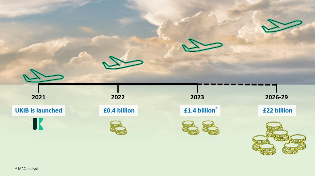
The UKIB: A New Force for Economic Growth?

Explore how the UK Infrastructure Bank is shaping the UK’s green and economic transformation. This article reviews UKIB’s mandate, funding capacity, early investments, and risks, and assesses its potential to drive long-term, sustainable infrastructure growth.

Heading 1

Heading 2

Heading 3

Heading 4

Heading 5
Heading 6

Lorem ipsum dolor sit amet, consectetur adipiscing elit, sed do eiusmod tempor incididunt ut labore et dolore magna aliqua. Ut enim ad minim veniam, quis nostrud exercitation ullamco laboris nisi ut aliquip ex ea commodo consequat. Duis aute irure dolor in reprehenderit in voluptate velit esse cillum dolore eu fugiat nulla pariatur.

Block quote

Ordered list

  1. Item 1
  2. Item 2
  3. Item 3

Unordered list

  • Item A
  • Item B
  • Item C

Text link

Bold text

Emphasis

Superscript

Subscript

Excellence in Consumer Engagement

This publication outlines 10 fundamental principles for effective engagement, exploring how businesses and regulators can foster trust, enhance decision-making, and create mutually beneficial outcomes.

Heading 1

Heading 2

Heading 3

Heading 4

Heading 5
Heading 6

Lorem ipsum dolor sit amet, consectetur adipiscing elit, sed do eiusmod tempor incididunt ut labore et dolore magna aliqua. Ut enim ad minim veniam, quis nostrud exercitation ullamco laboris nisi ut aliquip ex ea commodo consequat. Duis aute irure dolor in reprehenderit in voluptate velit esse cillum dolore eu fugiat nulla pariatur.

Block quote

Ordered list

  1. Item 1
  2. Item 2
  3. Item 3

Unordered list

  • Item A
  • Item B
  • Item C

Text link

Bold text

Emphasis

Superscript

Subscript

Featured

This paper has been published on following other platforms

No items found.

I was delighted that MCC's work was completed on time, and within budget, helping us deliver important changes and improvements, to the benefit of our stakeholders. ​ MCC's report is published on the CCC website.

- Bea Natzler
Team Leader at Climate Change Committee, UK

I am delighted to recommend MCC Economics. Specifically, I worked closely with PJ, who helped us with our Nuclear and CCUS projects. PJ helped us develop new policies and answer questions from our stakeholders. ​​His support helped us deliver important changes and improvements, to the benefit of our stakeholders.

- Gordon Hutcheson
Head of Nuclear Policy at Ofgem, UK

MCC Economics has helped us better understand the most important issues for our stakeholders, including: charges, shareholder returns, debt payments and inflation impacts.

- Leila N. Nasr
Section Head at Department of Energy, Abu Dhabi

I am delighted to recommend PJ and his team at MCC Economics. We've been working together on National Policy Statements to help meet net zero targets for 2030 and 2050. We initially appointed MCC Economics to support us on offshore wind consultation analysis and have recently reappointed MCC Economics to undertake a larger consultation analysis role across all sectors, including hydrogen, CCUS and networks. I can confirm that PJ and his team have shown excellent spreadsheet skills, alongside very good project management, planning and analysis skills, helping us deliver important changes, and continuous improvements, to the benefit of our stakeholders.

- Amy McHugh
Head of Environment in the Energy Infrastructure Planning Policy, UK

I am delighted to recommend PJ and his team from MCC Economics. They helped us with our price controls for Heathrow airport and for NATS (En Route) plc (the air traffic services provider). Specifically, the MCC team helped us deliver important changes and improvements to our financial models and supporting policy documents, to the benefit of our stakeholders.

- Dan Rock
Head of Corporate Finance at CAA, UK

I am delighted to confirm that I worked with PJ on a retail project in 2015. The project helped stakeholders understand electricity costs and charges. Specifically, the project helped us explain to stakeholders, internally and externally, why electricity charges differed across the regions (GB, NI & Ireland). PJ was a key member on the project team, which helped deliver changes and improvements in the understanding of energy retail.

- Kevin Shiels
Director at Utility Regulator, Northern Ireland