
Our comprehensive study on UAE GDP forecasting evaluates the effectiveness of three popular econometric models: ARIMA, VAR, and Linear Regression. Using real GDP data, the paper highlights each model's strengths and limitations over short-term and long-term horizons. The findings suggest that ARIMA is most effective for long-term forecasting, while Linear Regression shines in short-term, scenario-based predictions, provided accurate exogenous variable forecasts are available. Dive into this publication to gain valuable insights into forecasting methodologies that can enhance decision-making for businesses and policymakers in the UAE's dynamic economic landscape.
Forecasting GDP is crucial for economic planning and policymaking. This study compares the performance of three widely-used econometric models—ARIMA, VAR, and Linear Regression—using GDP data from the UAE. Employing a rolling forecast approach, we analyze the models’ accuracy over different time horizons. Results indicate ARIMA’s robust long-term forecasting capability, LR models perform better with short-term predictions, particularly when exogenous variable forecasts are accurate. These insights provide a valuable foundation for selecting forecasting models in the UAE’s evolving economy, suggesting ARIMA’s suitability for long-term outlooks and LR for short-term, scenario-based forecasts.
Rodrigo Malheiros Remor
MCC Economics & Finance
Abu Dhabi, UAE
PJ McCloskey
MCC Economics & Finance
Abu Dhabi, UAE
Abstract— Forecasting GDP is crucial for economicplanning and policymaking. This study compares theperformance of three widely-used econometric models—ARIMA, VAR, and Linear Regression—using GDP data fromthe UAE. Employing a rolling forecast approach, we analyze themodels’ accuracy over different time horizons. Results indicateARIMA’s robust long-term forecasting capability, LR modelsperform better with short-term predictions, particularly whenexogenous variable forecasts are accurate. These insightsprovide a valuable foundation for selecting forecasting modelsin the UAE’s evolving economy, suggesting ARIMA’s suitabilityfor long-term outlooks and LR for short-term, scenario-basedforecasts.
Keywords— GDP forecasting, ARIMA, VAR, LinearRegression, UAE economy
Gross Domestic Product (GDP) is a widely used measure of an economy’s performance. It is the sum of everything that is produced within an economy during a given period (Mankiw, 2022). Many businesses and government entities rely on GDP as a key parameter in their decision making. Central banks, for example, use this metric in their macroeconomic models, while businesses guide their investment decisions by, among other factors, their expectations on the future of the economy. This means that forecasts of likely movements in GDP are an important metric for many organizations.
This importance is evidenced by the number of different forecasting econometric models that have been developed over the decades in academia and the private and public sectors. Researchers have proposed many different time-series models such as Vector Autoregressive (VAR) (Robertson and Tallman, 1999; Roush et al., 2017; Bäurle et al., 2020), Autoregressive Integrated Moving Average (ARIMA) (Muma and Karoki, 2022; Yao Ma, 2024; Abdullah Ghazo, 2021), Long Short-Term Memory (LSTM) (Ouaadi and Ibourk, 2022; Zhang et al., 2023), among others, to measure and forecast GDP. Macroeconomic models have also been used to this end, using techniques such as Linear Regression (LR) (Chen, 2023) and Principal Component Analysis (PCA) (Alkhareif, 2018).
In this paper, we explore and compare the performance of 3 of these more popular approaches that have been successfully deployed for different economies and are widely accepted in the literature, namely the VAR, ARIMA, and LR models. We use United Arab Emirates’ (UAE) data to estimate these models and test their statistical properties and forecasting power, to determine which one is more suitable to the country. Our goal is to compare these three simple and inexpensive approaches, which can be easily implemented by any entity in their models and decision-making tools.
In the next section, we will explore the current literature on forecasting country GDP with these three methods. In section III, we explain each approach and estimate the best performing models. Section IV presents a comparison of their forecasting power. Finally, in section V we present our conclusions and suggest possible paths for future studies in this topic.
The academic literature has a wide range of work on different methods to forecast GDP and other macroeconomic variables. Yao Ma (2024) and Abdullah Ghazo (2021) developed ARIMA models for GDP forecasting in China and Jordania. Robertson and Tallman (1999), Roush et al. (2017) and Bäurle et al. (2020) show that VAR models can be used with many different arrangements of variables. Conversely, Ziyuan Chen (2023) shows that LR models can also be used to forecast GDP, suggesting that time-series approaches are just one of several possible forecasting methods.
The ARIMA methodology was developed by Box and Jenkins in 1976. It continues to be largely utilized in efforts to forecast GDP, because of its simplicity and its position as a useful benchmark to compare other models.
Muma and Karoki (2022) conducted a meta-review of 10 ARIMA models developed over the previous decade that were used to model and forecast the GDP of 8 different countries. TABLE I. summarizes the studies that the authors selected.
TABLE I. SELECTED PAPERS BY MUMA AND KAROKI
The authors noted that ARIMA models were effective in accurately modelling and forecasting GDP in the analysed studies, and recommended an individualized approach to estimating these types of models for each economy. They argue that the model estimation should take into consideration the country’s individual characteristics.
Yao Ma (2024) found a different ARIMA model than the one in TABLE I. for China, using annual GDP data from 1978 to 2022. Ma tested the specifications ARIMA (1,2,0) and ARIMA (0,2,0), and found the latter to be more statistically sound. Ma demonstrated that the model could be used to forecast GDP growth and concluded that it had a high accuracy for short-term forecasts. It is likely that a change in economic conditions between the period studied by Ma (2024) and the period studied by Yang et al (2016), which includes the recent pandemic shock, is the main explanation for their different results.
Abdullah Ghazo (2021) developed ARIMA models for Jordania’s GDP and Consumer Price Index (CPI) and found that the optimal specification for the production indicator was ARIMA (3,1,1). The author’s results show that the model was accurate for short-term forecasts, but less so for the long term.
The evidence present in the literature shows that the ARIMA methodology is effective in measuring GDP and relatively accurate in forecasting in the short term. Given the wide sample of countries covered by the literature, an ARIMA model is a promising candidate for the UAE.
The VAR model was introduced by Christopher Sims in 1980. Since then, it has been a major tool for macroeconomic analysis and forecast, along with its variations, among which the Bayesian VAR (BVAR) and the Structural VAR (SVAR). Applications of VAR models to forecast GDP usually make use of other major macroeconomic variables, such as CPI and unemployment rates (Robertson and Tallman, 1999; World Bank, 2020), or the GDP components themselves, whether arrived at by expenditure, income or production approaches (Roush et al., 2017).
In the paper published by the World Bank (2020), several VAR specifications were tested to forecast the GDP of Moldova. The authors tested a total of 34 variables, including the GDP and other economic indicators from the country’s main trade partners, to find the best specification. The authors forecasted 4 quarters ahead and used the Root Mean Square Error (RMSE) as their accuracy metric when comparing their best models’ forecasting power and their performance relative to a benchmark random walk model for the GDP. According to this metric, the best performing VAR model was a VAR(2) which used the GDP of Saudi Arabia and that of Russia in its specification, along with a quarter over quarter variation of the Moldavian GDP, reflecting the high interrelationships these two economies. The RMSE for that model was averaged at 2.16 in the 4 periods.
Robertson and Tallman (1999) used domestic economic indicators in their VAR model for the United States (US) economy, namely the US CPI, unemployment rate, a commodity price index, the Effective Federal Funds Rate and the M2 money stock. The last two variables were included envisioning the usage of the model by the president of the Federal Reserve Bank of Atlanta. The authors noted that the model’s user and the forecast’s purpose are important factors to decide how to specify the model and which approach to use.
The authors developed a monthly VAR(13), and used it to calculate quarterly and annual GDP forecasts on a rolling window of 11 years. The forecasts for the first 2 quarters presented an average RMSE of 3.05, while that for the first 2 years was 2.33. Their approach shows that different frequencies can also yield good results in VAR estimations.
Roush et al. (2017) found a quarterly VAR(4) to perform better for the US economy, among their tested models. The authors used an approach that focused on the expenditure components of GDP. They used in their model the real Personal Consumption Expenditure, real Government Consumption Expenditure and Gross Private Domestic Investment, as they directly relate to each of the domestic components of the GDP calculation. Also using quarterly data, they forecasted 6 periods ahead, concluding that due to the large confidence interval for farther quarters, the model is more useful to predict only one or two periods ahead.
Bäurle et al. (2020) chose the production side of the GDP calculation to specify their model estimations for Switzerland and the euro area. Among other similar approaches, the authors estimated a quarterly VAR(4) for each of the areas, using their respective sectoral GDP, which measures each sectors Gross Value Added (GVA). Their VAR model presented an RSME of 1.86 over the first 2 quarters, and of 1.90 over the first 8 quarters for Switzerland, and 2.25 and 2.23 over the same windows for the euro zone.
In this paper, we will follow Bäurle’s approach and use the sectoral GVA to estimate our VAR model, applying the production approach to calculate GDP.
Albeit less common, we can also find in the literature examples of LR being used not only to model GDP, but also to forecast it. These models usually make use of an underlying economic theory and rely on secondary forecasting models or the collection of external forecasts for the exogenous variables.
One recent example by Ziyuan Chen (2023) uses a multivariate linear regression model to forecast GDP, supported by univariate linear regression models and the growth retardation model to forecast the exogenous variables. The author adopted the variables GDP, population, labour force population, education investment and fixed asset investment, basing the estimation on an augmented Cobb-Douglas Function, which includes population growth and human capital in the classical Capital and Labour model specification.
The first step of this forecast is to establish the future values of population, using the growth retardation model, to then feed them to the estimated model between labour force population and total population to forecast the former. After this calculation, the author estimates two univariate trend models, using the year as the exogenous variable and education investment and fixed asset investment as the dependent variables. The resulting models are then used to calculate the future values of these variables. Finally, the author employs these future values in the GDP model and calculates the GDP forecast for a 20-year period.
Due to no accuracy measures being calculated in the paper, it is difficult to stablish if this approach yields good forecasts. The comparative nature of this paper will lead us to go further in our analysis and calculate these metrics.
Our paper contributes to expand the literature on comparisons of different estimation methods for GDP forecasting. We highlight 3 examples of similar comparisons.
Shahini and Haderi (2013) estimated four different models to forecast the quarterly GDP for Albania. TABLE II. shows the comparison of the authors’ results. The presented metrics, namely Bias, Standard Error (SE), Mean Squared Forecast Error (MSFE), Root of Mean Squared Forecast Error (RMSFE) and Mean Average Percentage Error (MAPE) evidently point to the VAR being the best approach to model and forecast GDP.
TABLE II. COMPARISON OF AUTHORS’ RESULTS
Josué R. Andrianady (2023) conducted a comparisonbetween ARIMA, VAR and MIDAS models’ forecasts ofMadagascar’s GDP. TABLE III. summarizes the accuracy ofthe three models the author estimated. In this case, the metricspoint to the ARIMA model being the best one for forecastingGDP, indicating that the differences of the characteristics ofAlbania and Madagascar’s economies prescribe differentmodels for an optimal GDP forecas
TABLE III. AUTHOR’S MODEL RESULTS
Following the same line of research, Maccarrone et al.(2021) compared the K-Nearest Neighbour (KNN) machinelearning algorithm to ARX, SARIMAX and LinearRegression (LR) models, while using AR and SARIMA asbenchmarks for the time series models, using US GDP datafor their estimations. According to the accuracy metricAverage Mean Squared Error (MSE), the best econometricmodel the authors found was LR, with a performance secondonly to the Machine Learning model.
The evidence presented above shows that many modelsmay be used to forecast GDP, and different economies mayfind better results in different models, depending on theirindividual characteristics and the data available for them. This Reinforces the importance of our effort to test which of thesethree approaches is better suited to forecast UAE’s GDP.
For this paper, we have selected our variables from adataset with 426 variables, to estimate the models of interest.This dataset ranged from general macroeconomic variables(e.g. inflation, unemployment, GDP, etc.) to sector-specificvariables (e.g. number of new business licenses, number ofhotel guests, oil production, etc.). TABLE IV. shows thenumber of variables available, by data source and the countryto which they belong.
TABLE IV. SELECTED PAPERS BY MUMA AND KAROKI
Due to data availability, the frequency of the variablessummarized above is annual and all the models are estimatedon this base, to ensure comparability. The variables used ineach of our model estimations underwent transformations such as differencing, standardization or indexation, to avoid distorted results. The transformations are delineated on the appropriate sections below.
The ARIMA models, denoted ARIMA(p,d,q), are structured around three components. The first an Autoregressive component (AR), which specifies how many lags of the variable are going to be used to explain their current value. This number is denoted p in the ARIMA notation. The second is the Integration component (I), which specifies how many times the variable is differenced, usually until it reaches stationarity. It is shown as d in the ARIMA notation. The third and last is the Moving Average component (MA), which specifies the arithmetic average of past residuals as parameters in the model. The residual lags used are given by q in the ARIMA notation.
A general ARIMA(p,d,q) is given by the equation:
Δᵈyₜ = β₀ + β₁yₜ₋₁ + β₂Δᵈyₜ₋₂ + … + βₚΔᵈyₜ₋ₚ + uₜ + θ₁uₜ₋₁ + θ₂uₜ₋₂ + … + θquₜ₋q
Where Δ denotes differencing, yₜ is the variable of interest on period t, βᵢ and θⱼ are the estimated parameters and uₜ is the model residual for period t.
For this model, we collected real GDP data for the UAE from 1975 to 2023, in local currency (Arab Emirates Dirhams - AED). This variable was collected from the UAE Federal Competitiveness and Statistics Centre’s (FCSC) data centre. Before estimating the model, we performed stationarity tests and analysed the data.
Starting with visual analysis, we plotted the Autocorrelation Function (ACF) for GDP. Figure 1 shows the results. The slower and constant reduction of the ACF over the GDP lags indicates that the variable is likely non-stationary.
After differencing GDP and redoing these calculations itseems that the new series became stationary at a 10%confidence level. Given that at a 5% confidence level wecannot reject the base hypothesis that the differenced series isnonstationary, it might be beneficial to difference the GDPseries a second time. On the other hand, the ACF plot indicatesthat the series is stationary, with an autoregressive component AR(1).
Given these apparently conflicting results, it may be beneficial to test a higher integration and additiona lautoregressive components within our ARIMA estimations, by creating and comparing the results of different ARIMA specifications.
Going back to the visual analysis, the Partial Autocorrelation Function (PACF) of the original GDP series, presented on Figure 3, indicates that the model may benefit from a Moving Average component MA(1)
Given the results above and the models found in the literature, we decided to estimate 9 ARIMA specifications and use Akaike and Bayesian Information Criteria (AIC and BIC)to select which performs the best. To create a long rolling forecast period, we limited our train data to 1975 through2013, leaving 10 years for a robust accuracy test. The specifications chosen along with their AIC and BIC are presented in TABLE V.
Based on both the AIC and the BIC, the specification ARIMA (1,2,1) seems to be the most well suited for the annual UAE GDP and is thus the one we chose to adopt.
VAR models, denoted VAR(p), are an extension of AR models (Roush et al., 2017), where every variable is considered and treated as endogenous. This means that for m variables, m models are estimated, each with a different variable as dependent and the p lags of itself and all the other variables as independent.
A general VAR(p) with m variables is represented by the system of equations:
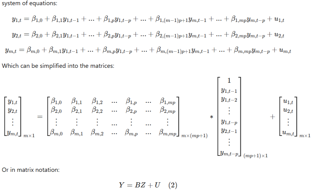
Where Y is the mx1 matrix containing all dependent variables, B is the mx(mp+1) matrix containing all the model coefficients, Z is the (mp+1)x1 matrix containing the p lags of every variable in the model and U is the mx1 matrix containing all the residuals. When estimating a VAR model, it is necessary to ensure that all the variables used are stationary, as to avoid a spurious regression.
Following the work of Bäurle et al (2020), we used sectoral GVA along with GDP data for the UAE from 1975 to 2023 in constant 2014 prices and local currency (AED). We also collected this data from the FCSC data centre. To ensure stationarity and maintain the interpretability of the model and the forecasts, we estimated the VAR models with the percentage change of the variables, calculated by:
Δyₜ = (yₜ − yₜ₋₁) / yₜ₋₁ (3)
This changed the interpretation of our model, but the forecast accuracy was kept comparable after a re-transformation of the forecasted values later, back to GDP level.
Before estimating the model, we did a correlation analysis of each sector against GDP, to reduce the number of parameters and increase the degrees of confidence by eliminating sectors with too low of a correlation to GDP. We chose 20% as a threshold for this selection. TABLE VI. showsthe calculated correlations.
TABLE VI. SECTOR CORRELATIONS TO GDP
We then estimated a VAR(1) and VAR(2), also using data from 1976 to 2013. The results and their criteria are summarized below.
TABLE VII. INFORMATION CRITERIA FOR VAR SPECIFICATIONS
While the VAR(1) has a lower BIC, VAR(2) has a lower AIC. This indicates that even though VAR(1) is better at explaining GDP, VAR(2) should be better at forecasting. Due to this ambiguity, and to ensure we are comparing the best results of each approach, we kept both models to be used for forecasting and used their accuracy metrics to determine which is best fitted for our purpose. This part of the analysis is outlined in section IV.
Linear Regression establishes the linear relationship between the independent and the dependent variables through Ordinary Least Squares (OLS) (Stock and Watson, 2020). A general LR model with k exogenous variables is represented by the equation:
y = β₀ + β₁x₁ + β₂x₂ + … + βₖxₖ + u (4)
Where y is the dependent endogenous variable, xᵢ are the independent exogenous variables, βᵢ are the coefficients estimated by OLS and u is the residual term. To estimate a LR using time-series variables, we also need to ensure their stationarity to avoid spurious regressions.
Due to a lack of availability of past values of the variables considered for the model, we had to reduce our observation period to 1990 through 2021. To compensate for the reduction in observations, we have extended our model training period to 2016, leaving 5 years for the out-of-sample testing. TABLE VIII. presents key information on the pre-selected variables.
TABLE VIII. LR VARIABLES’ INFORMATION
To avoid a multicollinearity issue, we have performed acorrelation analysis to assess whether some variables had tobe tested separately. We found that the only large correlationbetween the independent variables is approximately 84%,between “Exports” and the “Global Oil Prices”, which meansthat aside from monitoring the behaviour of these variables,multicollinearity should not be a concern in our estimation
The practical nature of our goal led us to adopt data miningprinciples to selecting the variables, as opposed to a purelytheoretical approach. The model was estimated as amultivariate linear regression, using Ordinary Least Squares(OLS), making use of current and lagged values of each of theselected variables. Through multiple iterations of the modelestimation, and through significance testing, we narrowedthese variables down to the ones that held the mostexplanatory power and led to a more statistically sound model.A summary of the resulting model is presented below.
We noticed that despite the small t-value of the second lagof Interest Rate, it contributed heavily to the model, both interms of explanatory power, as measured by the Adjusted 𝑅2,and model significance, as measured by the F-statistic. Sinceour goal is to forecast GDP growth, and not necessarilyexplain it, we decided to test the forecast accuracy of twomodel specifications: the one presented above (Model 1) andanother one dropping the second lag of Interest Rate andadding Imports, keeping only statistically significant variablesat a 10% significance level. The second model’s (Model 2)results are presented below.
The goal of this paper is to compare the forecasting power of these three approaches over shorter and longer horizons. For the short period, we calculated a one-year rolling forecast, meaning that we used each model to forecast one year ahead, re-estimated the model with the newer observations, and forecasted the following year, repeating this process throughout out testing window.
For the long period, we computed a five-year rolling forecast, meaning that we calculated the GDP forecast for the following 5 years after the model estimation, re-estimated the model adding one year of observations to the training dataset, and forecasted 5 years ahead, repeating the process throughout our testing window. For the ARIMA and VAR models, this process was performed 6 times, whereas for the LR model, due to the smaller test dataset, we could only repeat it 3 times at most.
For the LR model, since we wanted to estimate its accuracy in forecasting GDP and not in the forecasts of the exogenous variables, we assumed a “perfect prediction” of our explanatory variables, using their real-world values for calculating the GDP forecast. For a comprehensive assessment of the model’s viability, we also used a “naive” 5-year moving average of each of the exogenous variables to understand the GDP forecasts it could achieve when there is no information available on expected values of the future of the explanatory variables. For the “perfect prediction”, due to the data availability, we could only perform one 5-year forecast, while for the “naive prediction”, we did the forecast through three 5-year windows.
Figure 4 shows the forecast results of each model for the latest 5-year window (2019-2023) against real GDP. After the drop in GDP in 2020 due to the Covid-19 pandemic, our forecasts seem to match closely the inclination of the GDP curve, indicating that despite the tendency to overestimate the GDP levels, they seem to follow the variable’s behaviour quite closely. The exception is the ARIMA model forecast, which continues following the pre-pandemic trend of the variable, leading to a closer forecast of the post-recovery period in 2022 and 2023. This suggests that the ARIMA has a better long-term accuracy, but may not be the best performer in the short-term.
If the 2020 pandemic caused a structural break in the annual GDP time-series instead of a temporary fluctuation, we should expect the behaviours and performances of each model to be impacted in different ways. Such a possibility will need to be tested once there are more observations available, and if found true, the model specifications should be re-tested in light of the new evidence, and re-estimated to account for the new behaviour of GDP, if necessary.
At each iteration of the forecasts, we calculated their Mean Absolute Percentage Error (MAPE), in order to track the consistency of the model’s accuracy. The MAPE measures the average magnitude of the forecast error, as a percentage of the observed value of the variable. Its formula is given by equation 5. For the final comparison between the models, we calculated the average of their MAPE for all forecast periods.
MAPE = (1/n) ∑ from t=1 to n [ |yₜᴳ - yₜ| / yₜ ] * 100 (5)
The MAPE for each model on the 5-year forecast windows is presented in TABLE IX. As we can see, the time-series models performed better in the 5-year rolling forecasts. Among the VARs, VAR(2) had more accuracy overall and more consistency in its accuracy over all iterations. The best forecasts were given by the ARIMA (1,2,1), which had the lowest average MAPE at 5.2%.
It is worth noting that the average MAPEs of the LR models and the time-series models are not directly comparable, as the number of iterations calculated is lower forthe first group. However, comparing their range of resultsgives us a clear indication that the LR models’ performance isoverall worse in forecasting GDP in the longer term. For allthe models, except the VARs, the higher MAPEs wereobserved in the forecast period of 2017-2021. This could bean impactful factor in the LR models underperformance, asthis period was the only iteration of the “perfect prediction”forecasts, and one of the three in the “naïve prediction”forecasts. In the VARs, the highest MAPEs were observed inthe forecast of the period 2016-2020
TABLE IX. 5-YEAR FORECASTS MAPES
The 1-year rolling forecasts presented in TABLE X. show a different dynamic. While the ARIMA model still has more accuracy in terms of Average MAPE, we can see that the LRmodel 1 is more consistent in its accuracy, with the MAPE range of the “perfect prediction” being smaller than any other model. The difference between the results of the two prediction methods for the explanatory variables, however, shows that having accurate forecasts for each independent variable is very important for the model’s performance.
The VAR models show the widest range in results, with the VAR(1) specification performing better than the VAR(2)on average. This indicates that the approach is accurate, but inconsistent, and thus does not form a very good basis ford ecision making, especially considering the better performance of other approaches both in the short and longer terms.
TABLE X. 1-YEAR FORECASTS MAPEs
Forecasting GDP is not an easy task. It is affected by many factors, and tends to be easily swayed by external shocks, which are often unforeseeable. Several models have been created and modified to this end over the years, and as computing technology evolves, the tendency is that new models continue to be developed. Still, it is important that we understand whether the models we already have available are sufficient to this task, and among them which ones perform better at the application for which they are adopted.
We tested three approaches that are well documented in the literature, to determine which performed better in forecasting the UAE’s GDP, both in the short-term and long-term. We found that for 5-year windows, the ARIMA methodology, under the specification ARIMA (1,2,1) was the best performer, followed by the VAR methodology, under the specification VAR(2). Although both models present a higher accuracy, their disadvantage lies in the fact that they are backward-looking, and thus they don’t respond to changes in the expected behaviour of economic factors.
The LR models could provide this flexibility in reflecting expected scenarios in their forecasts. The advantage of this flexibility can be seen in model 1’s consistently high short-term accuracy, in the scenario where it is fed with perfect predictions of the explanatory variables. The difference in performance between the “Naive” and “Perfect” predictions-driven forecasts indicates that the performance of the explanatory variables forecasts is very important for this kind of model, which could present an issue if there is no way to access or perform accurate predictions on these variables.
Overall, our forecast results suggest the simultaneous use of different models for forward-looking decision making in the UAE. Specifically, the use of a LR model for short-term decisions, provided there is a good source for accurate predictions of the explanatory variables, and an ARIMA model for long-term decisions. This would provide the user with consistent metrics for their needs through many horizons.
Once the number of post-pandemic annual observations of GDP increases sufficiently, a study should be conducted to determine whether this event caused a structural break in the time-series or if it only led to a temporary shock. In case a structural break is determined to have occurred, all GDP forecasting models for the UAE should be re-tested and updated, including the ones presented in this paper. The new model estimations should place greater emphasis on the post-break behaviour of GDP.
Additionally, it would be beneficial to test which of the models estimated in this paper reacts most quickly to this break. This result could support the deployment of a specific model whenever a sudden break is believed to have occurred. This would lend the user more confidence in the forecast results over different economic conditions. Alternatively, testing the forecast performance of the models over steady-state periods and structural break periods separately may allow for a more thorough model selection which will depend not only on the forecast horizon, but also on the current state of the economy.
The adoption of alternative variables in the LR and VAR models, along with additional testing over larger time frames or at a higher frequency, should be considered in future studies. This will help assess whether their underperformance in the longer term is inherent to the approaches or if it is due to the specificities of these variables and time frame. Using higher frequencies will also allow for testing for a structural break in the GDP series sooner, as there will be more observations to use in the same time frame.
Different approaches and variables should also be tried and compared to the ones estimated here. Some suggestions would be LSTM models, PCA models, and Machine Learning approaches, all of which have little to no testing for forecasting UAE’s GDP in the literature. Modifications of the models presented in this paper, such as ARIMAX, VARX, BVAR and LVAR, should also be tested in future studies.
Finally, since we have two different approaches performing better over different horizons, it would be beneficial to understand what their tipping point is, meaning at what exact window does one model surpass the other, on average. We suggest that this work be done once other models have already been tried, since there may be other approaches than perform better in both horizons.
I was delighted that MCC's work was completed on time, and within budget, helping us deliver important changes and improvements, to the benefit of our stakeholders. MCC's report is published on the CCC website.

I am delighted to recommend MCC Economics. Specifically, I worked closely with PJ, who helped us with our Nuclear and CCUS projects. PJ helped us develop new policies and answer questions from our stakeholders. His support helped us deliver important changes and improvements, to the benefit of our stakeholders.

MCC Economics has helped us better understand the most important issues for our stakeholders, including: charges, shareholder returns, debt payments and inflation impacts.

I am delighted to recommend PJ and his team at MCC Economics. We've been working together on National Policy Statements to help meet net zero targets for 2030 and 2050. We initially appointed MCC Economics to support us on offshore wind consultation analysis and have recently reappointed MCC Economics to undertake a larger consultation analysis role across all sectors, including hydrogen, CCUS and networks. I can confirm that PJ and his team have shown excellent spreadsheet skills, alongside very good project management, planning and analysis skills, helping us deliver important changes, and continuous improvements, to the benefit of our stakeholders.

I am delighted to recommend PJ and his team from MCC Economics. They helped us with our price controls for Heathrow airport and for NATS (En Route) plc (the air traffic services provider). Specifically, the MCC team helped us deliver important changes and improvements to our financial models and supporting policy documents, to the benefit of our stakeholders.

I am delighted to confirm that I worked with PJ on a retail project in 2015. The project helped stakeholders understand electricity costs and charges. Specifically, the project helped us explain to stakeholders, internally and externally, why electricity charges differed across the regions (GB, NI & Ireland). PJ was a key member on the project team, which helped deliver changes and improvements in the understanding of energy retail.

.png)

Evidence-based analysis for transparent, defensible, and effective decision-making.
© All rights reserved – MCC Economics 2026.
.png)

%20(1).png)
.jpg)


